Initial Value Problem Differential Equation Solver
Greels
Mar 25, 2025 · 6 min read
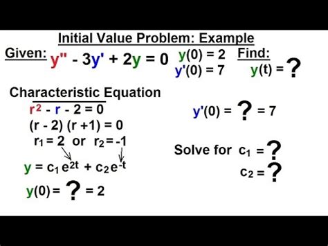
Table of Contents
Initial Value Problem Differential Equation Solvers: A Comprehensive Guide
Differential equations are the backbone of numerous scientific and engineering models, describing the rates of change in various systems. An initial value problem (IVP) is a type of differential equation where the solution is constrained by specifying the value of the dependent variable at a particular point, typically at the initial time. Solving these IVPs is crucial for understanding the behavior of the systems they represent. This comprehensive guide delves into the various methods used to solve initial value problems of differential equations, exploring their strengths, weaknesses, and applications.
Understanding Initial Value Problems
Before diving into the solving methods, let's solidify our understanding of IVPs. A first-order IVP generally takes the form:
dy/dx = f(x, y), y(x₀) = y₀
Where:
- dy/dx represents the derivative of the dependent variable 'y' with respect to the independent variable 'x'.
- f(x, y) is a function defining the relationship between 'x' and 'y' and their derivatives.
- y(x₀) = y₀ is the initial condition, specifying the value of 'y' at a starting point x₀.
Higher-order IVPs involve higher-order derivatives, but they can often be reduced to a system of first-order equations.
Numerical Methods for Solving IVPs
Analytical solutions for IVPs are not always possible, especially for complex functions f(x,y). This is where numerical methods come into play. These methods approximate the solution by iteratively stepping through the domain, using the initial condition and the differential equation to estimate the value of y at each step.
1. Euler's Method
Euler's method is the simplest numerical method for solving IVPs. It's based on the fundamental definition of the derivative:
dy/dx ≈ (y(x + h) - y(x)) / h
Where 'h' is the step size. Rearranging, we get:
y(x + h) ≈ y(x) + h * f(x, y)
This formula iteratively approximates the solution. While simple, Euler's method suffers from significant limitations: it's only first-order accurate (meaning the error is proportional to h), and it can be unstable for large step sizes or stiff equations (equations with rapidly changing solutions).
Advantages: Simple to understand and implement.
Disadvantages: Low accuracy, can be unstable, inefficient for complex problems.
2. Improved Euler Method (Heun's Method)
The Improved Euler Method, also known as Heun's method, is a second-order method that improves upon Euler's method by using a predictor-corrector approach. It first predicts the value at the next step using Euler's method, and then corrects this prediction using the average slope of the function at the current and predicted points.
Predictor: y* = y(x) + h * f(x, y)
Corrector: y(x + h) ≈ y(x) + h/2 * [f(x, y) + f(x + h, y*)]
This approach significantly reduces the error compared to Euler's method.
Advantages: More accurate than Euler's method, relatively simple to implement.
Disadvantages: Still less accurate than higher-order methods, can be inefficient for very complex problems.
3. Runge-Kutta Methods
Runge-Kutta methods are a family of powerful and widely used numerical methods for solving IVPs. They are higher-order methods, meaning they provide greater accuracy with smaller step sizes. The most common is the fourth-order Runge-Kutta method (RK4).
RK4 uses a weighted average of slopes at different points within the interval to estimate the next value of y. The formula is more involved but provides significantly improved accuracy.
k₁ = h * f(x, y)
k₂ = h * f(x + h/2, y + k₁/2)
k₃ = h * f(x + h/2, y + k₂/2)
k₄ = h * f(x + h, y + k₃)
y(x + h) ≈ y(x) + (k₁ + 2k₂ + 2k₃ + k₄) / 6
Advantages: High accuracy, relatively stable, widely applicable.
Disadvantages: More computationally expensive than lower-order methods, implementation is slightly more complex.
4. Adams-Bashforth Methods
Adams-Bashforth methods are multi-step methods, meaning they use information from previous steps to estimate the next value. They are explicit methods, meaning the next value is calculated directly without solving an equation. The accuracy increases with the number of previous steps used. However, a starting procedure like a Runge-Kutta method is needed to generate the initial values needed.
5. Adams-Moulton Methods
Adams-Moulton methods are also multi-step methods, but they are implicit methods. This means they require solving an equation to determine the next value. They typically offer higher accuracy than Adams-Bashforth methods for the same number of steps but involve more computation at each step.
6. Predictor-Corrector Methods
Predictor-corrector methods combine an explicit predictor method (like Adams-Bashforth) with an implicit corrector method (like Adams-Moulton). The predictor provides an initial estimate, which is then refined by the corrector. This approach improves accuracy and stability.
Choosing the Right Method
The choice of the most suitable method for solving an IVP depends on several factors:
- Accuracy requirements: For high accuracy, higher-order methods like RK4 or Adams-Moulton are preferred.
- Computational cost: Lower-order methods are less computationally expensive.
- Stiffness of the equation: Stiff equations require methods that are stable even with large step sizes, such as implicit methods.
- Complexity of the function f(x, y): Simple functions might only need Euler's method, while complex functions might require more sophisticated methods.
Software and Libraries
Several software packages and libraries are available to solve IVPs:
- MATLAB: Offers built-in functions like
ode45(a variable-step RK method) and others for various IVP solution methods. - Python (SciPy): The
scipy.integratemodule provides functions such assolve_ivp, which offers a wide range of solvers. - R: Packages like
deSolveprovide various functions for solving differential equations.
Applications of IVP Solvers
IVP solvers have a wide range of applications across numerous fields:
- Physics: Modeling projectile motion, planetary orbits, fluid dynamics, and many other physical phenomena.
- Engineering: Simulating the behavior of electrical circuits, mechanical systems, and chemical processes.
- Biology: Modeling population dynamics, disease spread, and other biological systems.
- Finance: Pricing options and other financial derivatives.
- Economics: Analyzing economic models and predicting market trends.
Advanced Topics
This guide has provided a fundamental overview. Further exploration could involve:
- Adaptive step size methods: Methods that adjust the step size during the computation to maintain accuracy and efficiency.
- Stiff equation solvers: Special methods designed to handle stiff equations efficiently and stably.
- Boundary value problems (BVPs): Problems where the solution is constrained by specifying values at both ends of the domain, requiring different solution techniques.
- Partial differential equations (PDEs): Equations involving multiple independent variables, requiring advanced numerical methods like finite difference, finite element, or finite volume methods.
Conclusion
Solving initial value problems is essential in numerous scientific and engineering applications. This guide has introduced the key numerical methods available, their strengths and weaknesses, and the factors influencing the choice of method. Understanding these methods empowers researchers and engineers to effectively model and analyze complex dynamic systems. While this provides a strong foundation, continuing your learning journey into more advanced methods and their practical application will significantly enhance your problem-solving capabilities. Remember to always consider the specific characteristics of your problem and select the most appropriate solver for optimal accuracy and efficiency.
Latest Posts
Latest Posts
-
How Many Ounces Is 17 G
Mar 26, 2025
-
How Much Is 58 Kilos In Pounds
Mar 26, 2025
-
How Many Miles Is 160 Km
Mar 26, 2025
-
How Many Feet Is 800 M
Mar 26, 2025
-
What Is 5 Percent Of 2000
Mar 26, 2025
Related Post
Thank you for visiting our website which covers about Initial Value Problem Differential Equation Solver . We hope the information provided has been useful to you. Feel free to contact us if you have any questions or need further assistance. See you next time and don't miss to bookmark.
