Step By Step Laplace Transform Calculator
Greels
Mar 22, 2025 · 5 min read
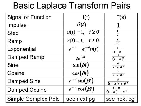
Table of Contents
A Step-by-Step Guide to Using a Laplace Transform Calculator
The Laplace transform, a powerful tool in mathematics and engineering, converts a function of time into a function of a complex frequency variable 's'. This transformation simplifies the solution of many differential equations, particularly those encountered in circuit analysis, control systems, and signal processing. While understanding the underlying mathematical principles is crucial, leveraging a Laplace transform calculator can significantly expedite the process and minimize errors. This comprehensive guide provides a step-by-step walkthrough of using such a calculator, explaining each step and offering insights into its practical applications.
Understanding the Laplace Transform
Before diving into calculator usage, let's briefly review the core concept. The Laplace transform of a function f(t), denoted as F(s), is defined by the integral:
∫₀^∞ e^(-st) f(t) dt
where:
- f(t) is the original function of time (often representing a signal or system response).
- s is a complex frequency variable (σ + jω, where σ is the real part and ω is the imaginary part).
- F(s) is the Laplace transform, a function of 's'.
The inverse Laplace transform, f(t) = L⁻¹{F(s)}, recovers the original time-domain function from its Laplace transform. This pair of transformations allows us to shift between time and frequency domains, simplifying complex problems.
Step-by-Step Guide to Using a Laplace Transform Calculator
The specific interface will vary depending on the calculator you choose (online or software-based). However, the fundamental steps remain similar. This guide assumes a general online calculator format.
Step 1: Identifying the Function
The first and most critical step is accurately defining the function you want to transform. This function, f(t), represents the time-domain signal or system response. Ensure you represent it correctly using mathematical notation. For example:
- Simple functions:
t,e^(-at),sin(ωt),cos(ωt),t²,t^n - More complex functions:
t*e^(-at),e^(-at)*sin(ωt),u(t)(unit step function)
Make absolutely certain your function is written correctly before proceeding; a single misplaced parenthesis or incorrect operator can lead to significant errors.
Step 2: Inputting the Function into the Calculator
Most calculators provide a text box or input field where you enter the function. Here, you'll input f(t) precisely as you defined it in Step 1. Be mindful of the specific syntax supported by the calculator. Many use standard mathematical notation, but some might require specific keywords or formatting. For example, the exponential function might be denoted as exp(), e^(), or simply e.
Step 3: Selecting the Transform Type
Some calculators allow you to specify whether you want the forward Laplace transform (time to frequency domain) or the inverse Laplace transform (frequency to time domain). Choose the appropriate option based on your needs.
Step 4: Executing the Calculation
Once the function and transform type are entered, click the "Calculate" or equivalent button. The calculator will process the input and perform the Laplace transform (or inverse transform). This might take a few seconds, depending on the complexity of the function and the calculator's processing power.
Step 5: Interpreting the Results
The calculator will present the result, F(s) (for the forward transform) or f(t) (for the inverse transform). This is the transformed function in the frequency or time domain, respectively. Carefully review the output to ensure it's in the expected format and make sense within the context of your problem.
Step 6: Verification (Optional but Recommended)
While the calculator automates the process, verifying the result is crucial, especially when dealing with complicated functions. You can use established Laplace transform tables or manual calculations (for simpler functions) to cross-check the accuracy of the calculator's output. Discrepancies might indicate errors in the input function or limitations of the calculator's algorithm.
Handling Different Function Types
Laplace transform calculators handle a variety of functions, but understanding how they treat different types is important:
1. Polynomial Functions: These are easily handled, with each term transformed individually. For example, t² + 2t + 1 transforms easily.
2. Exponential Functions: These are fundamental in many applications, with the transform of e^(-at) being 1/(s + a).
3. Trigonometric Functions: sin(ωt) and cos(ωt) transform into rational functions of 's'.
4. Unit Step Function (u(t)): This function is critical in representing signals that switch on at t=0. Its transform is 1/s.
5. Dirac Delta Function (δ(t)): This represents an impulse; its transform is simply 1.
6. Combined Functions: The calculator efficiently handles functions that are combinations of the above types, such as t*e^(-at)*sin(ωt). However, more complex functions might require simplification or decomposition before inputting them into the calculator.
Advanced Features and Considerations
Some advanced Laplace transform calculators might offer:
- Partial Fraction Decomposition: This is invaluable for simplifying complex rational functions resulting from the transform.
- Graphical Representation: Visualizing the transformed function in the s-plane (complex frequency plane) can offer valuable insights.
- Step-by-Step Solution: Some calculators display intermediate steps, helping users understand the transform process more deeply.
- Support for Different Notations: The ability to handle various notations for functions increases flexibility and convenience.
Applications in Engineering and Science
The Laplace transform's power lies in its broad applications across various fields:
- Circuit Analysis: Solving complex circuit problems involving resistors, capacitors, and inductors.
- Control Systems: Analyzing and designing control systems for stability and performance.
- Signal Processing: Analyzing and manipulating signals in the frequency domain.
- Mechanical Systems: Modeling and analyzing mechanical systems with various components like springs, dampers, and masses.
- Heat Transfer: Solving problems related to heat conduction and diffusion.
Conclusion
A Laplace transform calculator is an invaluable tool for engineers, scientists, and students working with differential equations and systems analysis. By following the step-by-step guide provided above and understanding the capabilities and limitations of the calculator, users can effectively leverage this powerful mathematical tool to simplify complex problems and gain deeper insights into the behavior of various systems. Remember to always verify the results and understand the underlying mathematical principles for a complete grasp of the topic. While calculators expedite the process, a solid understanding of the Laplace transform remains crucial for accurate interpretation and effective problem-solving.
Latest Posts
Latest Posts
-
How Many Ounces Is 90 Grams
Mar 23, 2025
-
Cuanto Es 86 Kg En Libras
Mar 23, 2025
-
How Many Feet Are In 360 Inches
Mar 23, 2025
-
How Many Feet In 4000 Meters
Mar 23, 2025
-
How Many Centimeters Are In 13 Inches
Mar 23, 2025
Related Post
Thank you for visiting our website which covers about Step By Step Laplace Transform Calculator . We hope the information provided has been useful to you. Feel free to contact us if you have any questions or need further assistance. See you next time and don't miss to bookmark.
