Step By Step Gaussian Elimination Calculator
Greels
Mar 25, 2025 · 6 min read
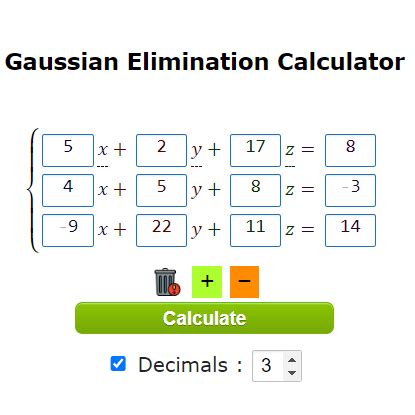
Table of Contents
Step-by-Step Gaussian Elimination Calculator: A Comprehensive Guide
Gaussian elimination, also known as row reduction, is a fundamental algorithm in linear algebra used to solve systems of linear equations. While software and online calculators can perform this process, understanding the underlying steps is crucial for grasping linear algebra concepts and troubleshooting potential issues. This guide provides a comprehensive, step-by-step walkthrough of Gaussian elimination, including how to use a hypothetical calculator to visualize the process.
Understanding Gaussian Elimination
Before diving into the calculator's use, let's review the core principles of Gaussian elimination. The goal is to transform an augmented matrix representing the system of equations into row echelon form (REF) or reduced row echelon form (RREF).
What is an Augmented Matrix?
An augmented matrix combines the coefficient matrix of a system of linear equations with its constant terms. For example, the system:
- x + 2y = 5
- 3x - y = 1
is represented by the augmented matrix:
[ 1  2 | 5 ]
[ 3 -1 | 1 ]
Row Echelon Form (REF):
A matrix is in REF if:
- All rows consisting entirely of zeros are at the bottom.
- The first non-zero element (leading coefficient) of each row is 1 (this is often, but not always, enforced).
- The leading coefficient of each row is to the right of the leading coefficient of the row above it.
Reduced Row Echelon Form (RREF):
RREF is a stricter form of REF. In addition to the REF requirements, RREF also mandates:
- Each leading coefficient is the only non-zero entry in its column.
Elementary Row Operations:
Gaussian elimination uses three elementary row operations to transform the augmented matrix:
- Swapping two rows: This doesn't change the solution of the system.
- Multiplying a row by a non-zero constant: This scales the equation but doesn't alter the solution.
- Adding a multiple of one row to another: This is a combination of equations, again preserving the solution.
Using a Hypothetical Gaussian Elimination Calculator
Let's imagine a "Gaussian Elimination Calculator" with the following features:
- Matrix Input: Allows users to input the augmented matrix of their system of equations.
- Step-by-Step Operation Selection: Presents a list of available row operations applicable to the current matrix state.
- Operation Execution: Executes the selected operation, updating the matrix accordingly.
- REF/RREF Check: Indicates whether the matrix is in REF or RREF.
- Solution Display: Displays the solution to the system of equations once the matrix is in RREF.
Step-by-Step Example using the Hypothetical Calculator
Let's solve the following system using our hypothetical calculator:
- 2x + y - z = 8
- -3x - y + 2z = -11
- -2x + y + 2z = -3
1. Matrix Input:
First, we input the augmented matrix:
[ 2  1 -1 | 8 ]
[-3 -1  2 |-11]
[-2  1  2 |-3 ]
2. Step-by-Step Row Reduction:
Our calculator might suggest the following steps:
Step 2.1: Making the leading coefficient of the first row 1.
The calculator suggests multiplying the first row by 1/2:
Calculator Operation: R1 -> (1/2)R1

[ 1  0.5 -0.5 | 4 ]
[-3 -1  2 |-11]
[-2  1  2 |-3 ]
Step 2.2: Eliminating the x-coefficient in the second row.
Next, the calculator suggests adding 3 times the first row to the second row:
Calculator Operation: R2 -> R2 + 3R1

[ 1  0.5 -0.5 | 4 ]
[ 0  0.5  0.5 | 1 ]
[-2  1  2 |-3 ]
Step 2.3: Eliminating the x-coefficient in the third row.
The calculator suggests adding 2 times the first row to the third row:
Calculator Operation: R3 -> R3 + 2R1

[ 1  0.5 -0.5 | 4 ]
[ 0  0.5  0.5 | 1 ]
[ 0  2  1 | 5 ]
Step 2.4: Making the leading coefficient of the second row 1.
The calculator suggests multiplying the second row by 2:
Calculator Operation: R2 -> 2R2

[ 1  0.5 -0.5 | 4 ]
[ 0  1  1 | 2 ]
[ 0  2  1 | 5 ]
Step 2.5: Eliminating the y-coefficient in the third row.
The calculator suggests subtracting 2 times the second row from the third row:
Calculator Operation: R3 -> R3 - 2R2

[ 1  0.5 -0.5 | 4 ]
[ 0  1  1 | 2 ]
[ 0  0 -1 | 1 ]
Step 2.6: Making the leading coefficient of the third row 1.
The calculator suggests multiplying the third row by -1:
Calculator Operation: R3 -> -R3

[ 1  0.5 -0.5 | 4 ]
[ 0  1  1 | 2 ]
[ 0  0  1 |-1 ]
Step 2.7: Eliminating the z-coefficient in the second row.
The calculator suggests subtracting the third row from the second row:
Calculator Operation: R2 -> R2 - R3

[ 1  0.5 -0.5 | 4 ]
[ 0  1  0 | 3 ]
[ 0  0  1 |-1 ]
Step 2.8: Eliminating the z-coefficient in the first row.
The calculator suggests adding 0.5 times the third row to the first row:
Calculator Operation: R1 -> R1 + 0.5R3

[ 1  0.5  0 | 3.5 ]
[ 0  1  0 | 3 ]
[ 0  0  1 |-1 ]
Step 2.9: Eliminating the y-coefficient in the first row.
The calculator suggests subtracting 0.5 times the second row from the first row:
Calculator Operation: R1 -> R1 - 0.5R2

[ 1  0  0 | 2 ]
[ 0  1  0 | 3 ]
[ 0  0  1 |-1 ]
3. Solution Display:
The calculator now displays the solution: x = 2, y = 3, z = -1. The matrix is in RREF.
Handling Special Cases
Gaussian elimination can encounter special cases:
-
Inconsistent Systems: If during the elimination process, you obtain a row of the form
[0 0 0 | c]wherecis a non-zero constant, the system is inconsistent and has no solution. -
Dependent Systems: If you end up with a row of all zeros, the system has infinitely many solutions. The variables corresponding to columns without leading 1s are free variables.
Advantages and Disadvantages of Gaussian Elimination
Advantages:
- Wide Applicability: Solves systems of linear equations of any size.
- Systematic Approach: Provides a clear, step-by-step method.
- Fundamental Algorithm: Underpins many other linear algebra algorithms.
Disadvantages:
- Computational Cost: Can be computationally expensive for very large systems.
- Numerical Instability: Susceptible to rounding errors in floating-point arithmetic, particularly for ill-conditioned systems.
Conclusion
Gaussian elimination is a powerful tool for solving systems of linear equations. While software and online calculators streamline the process, a deep understanding of the underlying steps is essential for effective problem-solving and error analysis. This guide, using a hypothetical calculator as a pedagogical tool, provides a clear and step-by-step approach to mastering this fundamental linear algebra technique. Remember to always check for special cases like inconsistent or dependent systems. With practice and understanding, you'll be proficient in using Gaussian elimination to tackle complex linear algebra problems.
Latest Posts
Latest Posts
-
How Many Inches Is 500 Mm
Mar 26, 2025
-
1 3 Lbs Is How Many Ounces
Mar 26, 2025
-
How Many Kilometers Is 6000 Miles
Mar 26, 2025
-
130 Mm Is How Many Inches
Mar 26, 2025
-
How Many Lbs Is 12 3 Oz
Mar 26, 2025
Related Post
Thank you for visiting our website which covers about Step By Step Gaussian Elimination Calculator . We hope the information provided has been useful to you. Feel free to contact us if you have any questions or need further assistance. See you next time and don't miss to bookmark.
