Solve The System Of Differential Equations
Greels
Mar 28, 2025 · 5 min read
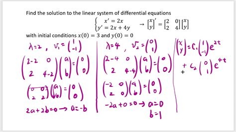
Table of Contents
Solving Systems of Differential Equations: A Comprehensive Guide
Solving systems of differential equations is a crucial aspect of many scientific and engineering disciplines. These systems describe the interconnected evolution of multiple variables over time or space. Understanding how to solve them is essential for modeling complex phenomena and predicting their behavior. This comprehensive guide delves into various methods for solving such systems, from simple techniques to more advanced approaches. We'll explore both linear and non-linear systems, focusing on practical applications and providing a solid foundation for further study.
Understanding Systems of Differential Equations
A system of differential equations involves two or more equations, each containing derivatives of multiple dependent variables with respect to one or more independent variables. The simplest case involves two first-order differential equations with two dependent variables and one independent variable, often time (t). This can be represented as:
dx/dt = f(x, y, t)
dy/dt = g(x, y, t)
where:
xandyare the dependent variables.tis the independent variable.f(x, y, t)andg(x, y, t)are functions defining the rates of change ofxandy.
Higher-order systems and systems with more than two variables can also be analyzed, often by converting them into a system of first-order equations.
Methods for Solving Systems of Differential Equations
Several methods exist for solving systems of differential equations, each with its strengths and limitations. The choice of method depends heavily on the nature of the equations – linear versus nonlinear, constant versus variable coefficients.
1. Elimination Method (for Linear Systems)
The elimination method is a powerful technique applicable to linear systems of differential equations. It involves manipulating the equations algebraically to eliminate one of the dependent variables, reducing the system to a single higher-order equation that can be solved using standard methods. Once the solution for one variable is found, it's substituted back into the original equations to solve for the other variable.
Example: Consider the system:
dx/dt + y = t
dy/dt - x = 1
We can differentiate the first equation with respect to t:
d²x/dt² + dy/dt = 1
Substituting dy/dt = x + 1 from the second equation gives:
d²x/dt² + x + 1 = 1
d²x/dt² + x = 0
This is a second-order linear homogeneous equation with constant coefficients, which can be solved using characteristic equations. The solution for x is then substituted back into one of the original equations to find y.
2. Substitution Method (for Linear and Non-linear Systems)
The substitution method involves expressing one dependent variable in terms of the other and substituting this expression into the remaining equations. This reduces the system's complexity, simplifying the solution process. This method is particularly useful for certain non-linear systems where other methods may be intractable.
Example: Suppose we have the system:
dx/dt = x + y
dy/dt = x - y
We can attempt to solve this system by expressing y in terms of x from the first equation and substituting into the second. However, this system lends itself more readily to methods described later.
3. Matrix Methods (for Linear Systems)
Matrix methods provide an elegant and efficient way to solve linear systems of differential equations. The system is represented in matrix form:
dX/dt = AX + B
where:
Xis a column vector of the dependent variables.Ais a constant coefficient matrix.Bis a column vector representing any forcing functions.
The solution involves finding the eigenvalues and eigenvectors of the matrix A. The general solution is then a linear combination of exponential functions involving these eigenvalues and eigenvectors. This method is particularly efficient for larger systems. Solving for homogeneous and non-homogeneous systems slightly differs, involving fundamental matrices and particular solutions.
4. Laplace Transform Method (for Linear Systems)
The Laplace transform is a powerful mathematical tool that transforms differential equations into algebraic equations, often simplifying the solution process. Applying the Laplace transform to each equation in the system yields a set of algebraic equations that can be solved for the Laplace transforms of the dependent variables. The inverse Laplace transform then gives the solutions in the time domain. This method is particularly advantageous for systems with discontinuous forcing functions.
5. Numerical Methods (for Linear and Non-linear Systems)
For complex systems that lack analytical solutions, numerical methods provide approximate solutions. Methods like Euler's method, Runge-Kutta methods (various orders), and predictor-corrector methods are commonly used. These methods involve discretizing the time or space domain and iteratively approximating the solution at each step. The accuracy of the solution depends on the step size and the chosen numerical method. Numerical methods are often implemented using computational software packages.
Applications of Solving Systems of Differential Equations
Systems of differential equations are fundamental in numerous scientific and engineering fields. Some key applications include:
- Physics: Modeling coupled oscillations, planetary motion, and fluid dynamics.
- Chemistry: Analyzing reaction kinetics and chemical equilibrium.
- Biology: Studying population dynamics (predator-prey models), epidemiology (disease spread), and neural networks.
- Engineering: Designing control systems, analyzing electrical circuits, and modeling mechanical systems.
- Economics: Describing economic growth models and market dynamics.
Advanced Topics
Beyond the basic methods discussed, several advanced techniques address more challenging systems:
- Nonlinear Systems: Solving nonlinear systems often requires more sophisticated methods like perturbation techniques, numerical methods, or qualitative analysis (phase plane analysis).
- Partial Differential Equations (PDEs): PDEs involve partial derivatives with respect to multiple independent variables. Methods like separation of variables, Fourier transforms, and finite element methods are used to solve them.
- Systems with Boundary Conditions: Many applications involve systems with boundary conditions specifying the values of the dependent variables at specific points in space or time. Solving these systems often requires specialized techniques.
- Stability Analysis: Understanding the stability of solutions is crucial in many applications. Linearization, Lyapunov functions, and other methods are used to analyze the stability of equilibrium points and solutions.
Conclusion
Solving systems of differential equations is a broad and challenging area with numerous applications. Mastering the various techniques presented here—from elimination and matrix methods to numerical approaches—provides a solid foundation for tackling a wide range of problems in science and engineering. The choice of the most appropriate method depends heavily on the specific characteristics of the system, its linearity, and the desired accuracy of the solution. Further exploration into advanced techniques will allow for the successful modeling and analysis of increasingly complex phenomena. Remember that the effective use of these methods often requires a strong understanding of linear algebra, calculus, and numerical analysis.
Latest Posts
Latest Posts
-
How Many Centimeters Are In 36 Inches
Mar 31, 2025
-
What Is 1 70 M In Feet
Mar 31, 2025
-
How Tall Is 194 Cm In Feet
Mar 31, 2025
-
How Tall Is 24 Inches In Feet
Mar 31, 2025
-
How Long Is 39 Inches In Feet
Mar 31, 2025
Related Post
Thank you for visiting our website which covers about Solve The System Of Differential Equations . We hope the information provided has been useful to you. Feel free to contact us if you have any questions or need further assistance. See you next time and don't miss to bookmark.
