Linear First Order Differential Equations Calculator
Greels
Mar 21, 2025 · 7 min read
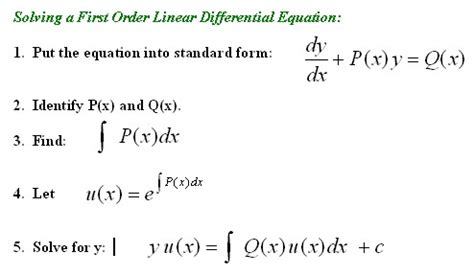
Table of Contents
Linear First Order Differential Equations Calculator: A Comprehensive Guide
Linear first-order differential equations are a cornerstone of many scientific and engineering disciplines. Solving them accurately and efficiently is crucial for a wide range of applications, from modeling population growth to predicting the behavior of electrical circuits. While analytical solutions exist, the complexity can often necessitate the use of computational tools, specifically, a linear first-order differential equation calculator. This comprehensive guide explores the nuances of these equations, explains their various solution methods, and provides insights into using calculators effectively for accurate and timely results.
Understanding Linear First-Order Differential Equations
A first-order differential equation involves a function and its first derivative. A linear first-order differential equation takes the general form:
dy/dx + P(x)y = Q(x)
Where:
dy/dxrepresents the first derivative of the function y with respect to x.P(x)andQ(x)are functions of x.
The linearity of this equation is crucial. It means that the dependent variable, y, and its derivative appear only to the first power and are not multiplied together. This characteristic simplifies the solution process significantly.
Key Characteristics and Significance
The significance of linear first-order differential equations stems from their widespread applicability across numerous fields:
- Physics: Modeling various physical phenomena, including radioactive decay, Newton's law of cooling, and the discharge of a capacitor.
- Engineering: Analyzing electrical circuits, mechanical systems, and fluid dynamics.
- Biology: Studying population growth, drug absorption, and the spread of diseases.
- Economics: Modeling economic growth, financial markets, and supply and demand.
- Chemistry: Analyzing chemical reactions and the rates of change in chemical concentrations.
Solving Linear First-Order Differential Equations: Analytical Methods
Before diving into calculator usage, it’s essential to understand the analytical methods for solving these equations. These methods form the basis of the algorithms employed within the calculators.
1. Integrating Factor Method
This is the most common and widely used technique. The integrating factor, denoted by I(x), is defined as:
I(x) = e^(∫P(x)dx)
Multiplying both sides of the original equation by the integrating factor transforms the left-hand side into the derivative of a product:
I(x)dy/dx + I(x)P(x)y = I(x)Q(x)
This simplifies to:
d/dx[I(x)y] = I(x)Q(x)
Integrating both sides with respect to x yields the general solution:
I(x)y = ∫I(x)Q(x)dx + C
Where C is the constant of integration. Solving for y provides the final solution.
2. Separation of Variables (Specific Cases)
If the equation can be manipulated into the form:
dy/dx = f(x)g(y)
Then the variables can be separated:
dy/g(y) = f(x)dx
Integrating both sides independently provides the general solution. Note that this method is only applicable to specific cases where the equation is separable. Many linear first-order equations are not directly separable.
The Role of a Linear First-Order Differential Equations Calculator
While analytical methods provide a fundamental understanding, solving complex equations manually can be tedious and prone to errors. This is where a linear first-order differential equation calculator becomes invaluable. These calculators automate the solution process, significantly reducing the time and effort required while minimizing the risk of calculation mistakes.
Choosing and Using a Linear First-Order Differential Equations Calculator
Several online calculators and software packages can solve linear first-order differential equations. The choice depends on your specific needs and preferences:
-
Online Calculators: Many free online calculators provide a quick and convenient way to solve these equations. Simply input the functions P(x) and Q(x), and the calculator provides the solution. However, these often lack advanced features and may not handle very complex functions.
-
Mathematical Software Packages (Matlab, Mathematica, Maple): These powerful tools offer more advanced capabilities, including symbolic solutions, numerical approximations, and visualization options. They are suitable for complex equations and research-level applications but require a deeper understanding of the software and potentially a cost for licensing.
-
Programming Languages (Python with SciPy): For users comfortable with programming, using languages like Python with libraries such as SciPy offers high flexibility and control. You can implement various numerical methods to solve the equation, providing customizability not found in simpler calculators.
Key Features to Look For:
- Ease of Use: The calculator should have a user-friendly interface that is easy to navigate and understand.
- Accuracy: The calculator should provide accurate results, especially when dealing with complex equations.
- Detailed Steps: Some calculators show the step-by-step solution process, which is helpful for learning and understanding the underlying mathematical concepts.
- Flexibility: The calculator should be able to handle a wide range of input functions, including those involving trigonometric, exponential, and logarithmic functions.
- Visualization: Advanced calculators might allow you to visualize the solution graphically, which can be valuable for understanding the behavior of the solution.
Using a Calculator Effectively:
- Input the Correct Functions: Accurately enter the functions P(x) and Q(x) into the calculator. Ensure you use correct notation and syntax.
- Specify Initial Conditions (if applicable): Many differential equations require initial conditions (a value of y at a specific x) to determine the particular solution. Provide these conditions as instructed by the calculator.
- Check the Results: Always verify the results obtained from the calculator using alternative methods or by hand-checking, especially for simple cases. This helps to ensure the accuracy of the calculation and identify any potential errors.
- Understand the Limitations: Calculators may have limitations in handling extremely complex or ill-defined equations. Be aware of these limitations and consider alternative approaches if necessary.
Numerical Methods for Solving Linear First-Order Differential Equations
When analytical solutions are impossible or impractical, numerical methods provide approximate solutions. These methods are frequently implemented within sophisticated calculators and software.
1. Euler's Method
This is a simple first-order numerical method that approximates the solution by stepping through small increments of x. The formula is:
y_(i+1) = y_i + h*f(x_i, y_i)
Where:
his the step size.f(x_i, y_i)is the value of the derivative at (x_i, y_i).
Euler's method is relatively simple to implement but can be inaccurate for large step sizes.
2. Improved Euler's Method (Heun's Method)
This method improves the accuracy of Euler's method by using a predictor-corrector approach. It first predicts the value of y at the next step using Euler's method, and then corrects this prediction using the average slope between the current and predicted points.
3. Runge-Kutta Methods
These are a family of higher-order numerical methods that offer greater accuracy than Euler's method. The most commonly used is the fourth-order Runge-Kutta method (RK4), which provides a good balance between accuracy and computational cost.
Advanced Applications and Considerations
The applications of linear first-order differential equations extend far beyond simple examples. Understanding how to use calculators efficiently is crucial when tackling more complex scenarios:
- Systems of Differential Equations: Many real-world problems involve multiple interacting variables, leading to systems of differential equations. Sophisticated calculators and software can handle such systems effectively.
- Partial Differential Equations: While this guide focuses on ordinary differential equations, many real-world problems are modeled using partial differential equations (PDEs). Numerical methods are often required to solve these, and specialized software is usually necessary.
- Boundary Value Problems: These problems specify the value of the solution at both ends of an interval, rather than just an initial condition. Solving these requires specialized techniques and software.
Conclusion
Linear first-order differential equations are fundamental to many scientific and engineering disciplines. While analytical solutions are ideal, the complexity of many problems necessitates the use of computational tools—specifically, a linear first-order differential equation calculator. Understanding the underlying mathematical principles, choosing the right calculator or software, and being aware of the capabilities and limitations of numerical methods are key to successfully solving these equations and applying them to real-world problems. The use of calculators should not be seen as a replacement for understanding the underlying mathematics but rather as a powerful tool to efficiently and accurately obtain solutions, allowing for a deeper focus on the interpretation and application of the results.
Latest Posts
Latest Posts
-
How Many Kg Is 205 Pounds
Mar 28, 2025
-
91 Kg Is How Many Pounds
Mar 28, 2025
-
120 Km Is How Many Miles
Mar 28, 2025
-
How Many Miles In 250 Kilometers
Mar 28, 2025
-
How Many Kilograms In 175 Pounds
Mar 28, 2025
Related Post
Thank you for visiting our website which covers about Linear First Order Differential Equations Calculator . We hope the information provided has been useful to you. Feel free to contact us if you have any questions or need further assistance. See you next time and don't miss to bookmark.
