Laplace Transform Step By Step Calculator
Greels
Mar 21, 2025 · 5 min read
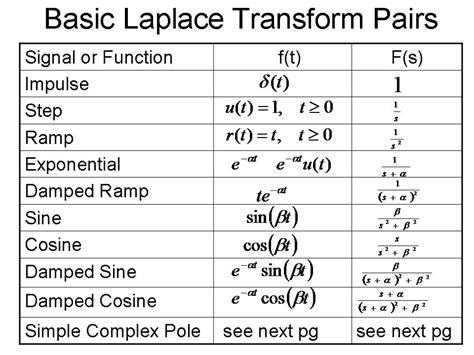
Table of Contents
Laplace Transform Step-by-Step Calculator: A Comprehensive Guide
The Laplace transform is a powerful mathematical tool used extensively in engineering, physics, and other scientific disciplines to solve complex differential equations. It transforms a function of time into a function of a complex variable, often simplifying the problem significantly. While the theoretical aspects of the Laplace transform can be challenging, the practical application is often streamlined with the help of calculators. This article delves into the intricacies of the Laplace transform, providing a step-by-step guide and exploring the functionalities of a hypothetical Laplace transform step-by-step calculator.
Understanding the Laplace Transform
Before we dive into using a calculator, it's crucial to understand the core concept. The Laplace transform of a function f(t), denoted as F(s), is defined by the integral:
ℒ{f(t)} = F(s) = ∫₀^∞ e^(-st) f(t) dt
Where:
- f(t) is the original function of time (often representing a system's response).
- s is a complex variable (s = σ + jω, where σ and ω are real numbers).
- F(s) is the Laplace transform of f(t), a function in the s-domain.
The integral transforms the function from the time domain (t) to the frequency domain (s). The beauty of the Laplace transform lies in its ability to convert differential equations into algebraic equations, which are significantly easier to solve. After solving in the s-domain, the inverse Laplace transform is applied to obtain the solution in the time domain.
Key Properties of the Laplace Transform
Several properties simplify the application of the Laplace transform. Understanding these properties is vital for efficient use of any Laplace transform calculator:
1. Linearity:
ℒ{af(t) + bg(t)} = aℒ{f(t)} + bℒ{g(t)} = aF(s) + bG(s)
This property allows us to transform linear combinations of functions individually and then combine the results.
2. Time Shifting:
ℒ{f(t - a)u(t - a)} = e^(-as)F(s), where u(t) is the unit step function.
This property is crucial when dealing with delayed or shifted signals.
3. Frequency Shifting:
ℒ{e^(at)f(t)} = F(s - a)
This simplifies the transformation of exponentially modulated signals.
4. Differentiation in Time Domain:
ℒ{f'(t)} = sF(s) - f(0)
ℒ{f''(t)} = s²F(s) - sf(0) - f'(0)
This allows us to transform differential equations into algebraic equations.
5. Integration in Time Domain:
ℒ{∫₀^t f(τ)dτ} = F(s)/s
This property is beneficial when dealing with integral equations.
The Hypothetical Laplace Transform Step-by-Step Calculator
Let's imagine a powerful, user-friendly Laplace transform step-by-step calculator. This calculator would provide a detailed breakdown of the transformation process, allowing users to understand not just the result but also the methodology.
Features:
-
Function Input: The calculator would accept a wide range of function inputs, including standard mathematical functions (sin, cos, exp, etc.), piecewise functions, and functions defined using mathematical notation. It would handle both continuous and discrete functions.
-
Step-by-Step Solution: This is the core feature. The calculator would not just provide the final Laplace transform; it would show each step of the calculation. This includes:
- Applying the definition of the Laplace transform (the integral).
- Using relevant properties (linearity, time shifting, etc.).
- Performing integration techniques (integration by parts, partial fractions, etc.).
- Simplification of the resulting expression.
-
Visual Representation: The calculator could provide visual aids such as graphs of the original function and its Laplace transform to enhance understanding. This would help users visualize the transformation process.
-
Inverse Laplace Transform: The calculator would also offer the inverse Laplace transform functionality, allowing users to obtain the time-domain solution from the s-domain result. This would involve a similar step-by-step process, including partial fraction decomposition (where applicable).
-
Error Handling: Robust error handling would be essential. The calculator should identify invalid inputs, inappropriate functions, and other potential issues, providing clear error messages to guide users.
-
Table of Common Laplace Transforms: A readily accessible table of common Laplace transforms would speed up the process for frequently used functions.
Step-by-Step Example using the Hypothetical Calculator
Let's illustrate the use of our hypothetical calculator with an example: Find the Laplace transform of f(t) = t²e^(-2t)u(t).
1. Function Input: The user would input the function: t^2 * exp(-2t) * u(t).
2. Step-by-Step Calculation (as displayed by the calculator):
-
Step 1: Applying the definition of the Laplace transform: The calculator would show the integral: ∫₀^∞ e^(-st) * t² * e^(-2t) dt
-
Step 2: Combining exponential terms: The calculator would simplify the integral to: ∫₀^∞ t² * e^(-(s+2)t) dt
-
Step 3: Applying the property for the Laplace transform of t^n: The calculator would use the formula ℒ{t^n} = n! / s^(n+1) and show the application to the specific case of t².
-
Step 4: Substitution and Simplification: The calculator would substitute and simplify the expression, showing the steps involved in arriving at the final result.
-
Step 5: Final Result: The calculator would display the final Laplace transform: 2 / (s + 2)³
3. Inverse Laplace Transform: The user could then use the calculator to find the inverse Laplace transform of the obtained result. Again, the calculator would provide a detailed step-by-step process.
Advanced Features for the Calculator
Advanced features could enhance the calculator's utility:
-
Support for systems of differential equations: The calculator could handle the Laplace transforms of systems of differential equations, a common scenario in many engineering problems.
-
Convolution theorem implementation: The calculator could implement the convolution theorem, which simplifies the calculation of the Laplace transform of the convolution of two functions.
-
Numerical methods integration: For cases where analytical integration is difficult or impossible, the calculator could employ numerical methods to approximate the Laplace transform.
-
User-defined functions: Allow users to define their own functions and apply the Laplace transform to them.
Conclusion
A step-by-step Laplace transform calculator would be an invaluable tool for students, engineers, and researchers. By providing a clear and detailed breakdown of the calculation process, such a calculator would enhance understanding and promote efficient problem-solving. While such a sophisticated calculator doesn't currently exist in a single, readily available form, the combination of existing mathematical software and online resources can often achieve a similar outcome. The future of mathematical computation lies in increasingly user-friendly and comprehensive tools that bridge the gap between theory and practical application. The detailed, step-by-step approach outlined here serves as a blueprint for developing such powerful and educational tools.
Latest Posts
Latest Posts
-
Find The Radius Of Convergence Calculator
Mar 28, 2025
-
How Tall Is 65inches In Feet
Mar 28, 2025
-
How Much Is 62 Inches In Feet
Mar 28, 2025
-
161 Cm To Inch And Feet
Mar 28, 2025
-
100 99 100 99 100 100
Mar 28, 2025
Related Post
Thank you for visiting our website which covers about Laplace Transform Step By Step Calculator . We hope the information provided has been useful to you. Feel free to contact us if you have any questions or need further assistance. See you next time and don't miss to bookmark.
