Laplace Transform Calculator Step By Step
Greels
Mar 24, 2025 · 5 min read
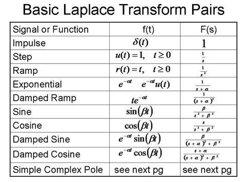
Table of Contents
Laplace Transform Calculator: A Step-by-Step Guide to Solving Complex Equations
The Laplace transform is a powerful mathematical tool used extensively in engineering and physics to simplify the solution of differential equations. It transforms a function of time into a function of a complex variable, often making complex problems significantly easier to solve. While the underlying mathematics can be intricate, understanding the process step-by-step can demystify the technique. This comprehensive guide will walk you through the Laplace transform process, explaining each step and providing examples to solidify your understanding. We'll cover both manual calculation and the use of online calculators to efficiently solve Laplace transforms.
Understanding the Laplace Transform
The Laplace transform, denoted by ℒ{f(t)}, converts a function of time, f(t), into a function of a complex frequency variable, s. The general formula is:
ℒ{f(t)} = F(s) = ∫₀^∞ e^(-st) f(t) dt
This integral transforms the function from the time domain (t) to the complex frequency domain (s). The key is that many differential equations become algebraic equations in the s-domain, greatly simplifying their solution.
Key Properties of the Laplace Transform
Before diving into step-by-step calculations, understanding the key properties of the Laplace transform is crucial. These properties significantly streamline the process:
- Linearity: ℒ{af(t) + bg(t)} = aℒ{f(t)} + bℒ{g(t)}, where 'a' and 'b' are constants. This allows us to break down complex functions into simpler components.
- Time Shifting: ℒ{f(t - a)u(t - a)} = e^(-as)F(s), where u(t) is the unit step function and 'a' is a constant. This handles delayed functions.
- Frequency Shifting: ℒ{e^(at)f(t)} = F(s - a). This is useful for handling exponentially decaying or growing functions.
- Differentiation in Time Domain: ℒ{f'(t)} = sF(s) - f(0) and ℒ{f''(t)} = s²F(s) - sf(0) - f'(0). This is the cornerstone of solving differential equations using Laplace transforms.
- Integration in Time Domain: ℒ{∫₀^t f(τ)dτ} = F(s)/s. This simplifies integral terms within differential equations.
Step-by-Step Guide to Manual Calculation of Laplace Transforms
Let's illustrate the process with a simple example: finding the Laplace transform of f(t) = t².
Step 1: Write the Laplace Transform Integral
We start with the definition:
ℒ{t²} = ∫₀^∞ e^(-st) t² dt
Step 2: Apply Integration by Parts
Integration by parts is frequently needed. The formula is: ∫u dv = uv - ∫v du
Let's choose:
- u = t² => du = 2t dt
- dv = e^(-st) dt => v = (-1/s)e^(-st)
Applying integration by parts once:
∫₀^∞ e^(-st) t² dt = [-t²e^(-st)/s]₀^∞ + (2/s)∫₀^∞ te^(-st) dt
The first term evaluates to 0 as t approaches infinity (assuming s > 0).
Step 3: Apply Integration by Parts Again
We need to apply integration by parts again to solve the remaining integral:
- u = t => du = dt
- dv = e^(-st) dt => v = (-1/s)e^(-st)
(2/s)∫₀^∞ te^(-st) dt = (2/s) * [(-te^(-st)/s)₀^∞ + (1/s)∫₀^∞ e^(-st) dt]
Again, the first term evaluates to 0.
Step 4: Solve the Remaining Integral
The final integral is straightforward:
(1/s)∫₀^∞ e^(-st) dt = (1/s) * [-e^(-st)/s]₀^∞ = 1/s²
Step 5: Combine the Results
Putting everything together:
ℒ{t²} = 0 + (2/s) * (1/s²) = 2/s³
Therefore, the Laplace transform of t² is 2/s³.
Step-by-Step Guide Using a Laplace Transform Calculator
While manual calculation is instructive, using a Laplace transform calculator significantly speeds up the process, especially for complex functions. Many online calculators are available; the process generally involves these steps:
Step 1: Find a Reliable Online Calculator
Numerous websites offer Laplace transform calculators. Ensure the calculator you choose has a clear interface and provides step-by-step solutions (if available).
Step 2: Input the Function
Carefully enter the function f(t) into the calculator's input field. Be precise with notation and use the correct mathematical symbols. Commonly used notations for functions may vary slightly between different calculators.
Step 3: Specify the Variable
Most calculators require you to specify the independent variable (usually 't' for time).
Step 4: Execute the Calculation
Click the "Calculate" or equivalent button to initiate the computation.
Step 5: Interpret the Results
The calculator will provide the Laplace transform F(s) of the input function. Many calculators will also offer a breakdown of the calculation steps, enabling a more in-depth understanding of the process. Pay close attention to any assumptions or limitations mentioned by the calculator.
Advanced Applications and Considerations
The Laplace transform finds its greatest utility in solving differential equations. This involves:
- Taking the Laplace transform of the differential equation: Use the differentiation properties to transform the derivatives into algebraic expressions.
- Solving the resulting algebraic equation: This will yield F(s).
- Taking the inverse Laplace transform: This involves finding the function f(t) that corresponds to F(s). Many online resources and calculators also offer inverse Laplace transforms. This step can sometimes require partial fraction decomposition, which is a method used to simplify complex rational functions into a sum of simpler fractions which are readily invertible.
Handling Different Types of Functions
Laplace transforms can handle a wide range of functions, including:
- Polynomials: The Laplace transforms of polynomials are readily obtained using the linearity property and the transform of tⁿ.
- Exponential Functions: These transforms easily using the frequency shift property.
- Trigonometric Functions: These also have straightforward transforms.
- Step Functions: These are handled using the time shift property.
- Impulse Functions: The Dirac delta function is an important function in signal processing and system theory, and its Laplace transform is 1.
Limitations and Considerations
- Convergence: The Laplace transform only converges for functions that satisfy certain conditions. Functions with exponential growth might not have a Laplace transform.
- Uniqueness: While the Laplace transform is unique for a given function under certain conditions, the inverse transform may not always be unique.
Conclusion
The Laplace transform is a powerful technique for simplifying the solution of differential equations. While manual calculations can be tedious for complex functions, online calculators offer efficient and accurate solutions. By understanding the step-by-step process and the key properties of the Laplace transform, you can effectively utilize this mathematical tool to solve a wide range of problems in various fields of science and engineering. Remember to always choose reliable online calculators and carefully interpret the results to avoid misunderstandings. Mastering the Laplace transform significantly enhances your ability to analyze and solve complex systems.
Latest Posts
Latest Posts
-
How Many Feet Is 53 In
Mar 26, 2025
-
What Day Will It Be In 48 Days
Mar 26, 2025
-
End Behavior Of Logarithmic Functions Calculator
Mar 26, 2025
-
What Is 125 Kg In Pounds
Mar 26, 2025
-
38 Lbs Bang Bao Nhieu Kg
Mar 26, 2025
Related Post
Thank you for visiting our website which covers about Laplace Transform Calculator Step By Step . We hope the information provided has been useful to you. Feel free to contact us if you have any questions or need further assistance. See you next time and don't miss to bookmark.
