Initial Value Problem Differential Equation Calculator
Greels
Mar 29, 2025 · 6 min read
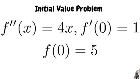
Table of Contents
Initial Value Problem Differential Equation Calculator: A Comprehensive Guide
Solving initial value problems (IVPs) for differential equations is a fundamental task in many scientific and engineering disciplines. These problems involve finding a function that satisfies a given differential equation and specific initial conditions. While analytical solutions are ideal, they're not always attainable. This is where numerical methods and, consequently, initial value problem differential equation calculators come into play. This article delves deep into the world of IVP solvers, exploring their applications, underlying methods, limitations, and how to effectively utilize online calculators and software packages.
Understanding Initial Value Problems (IVPs)
An initial value problem consists of a differential equation and a set of initial conditions. The differential equation describes the relationship between a function and its derivatives, while the initial conditions specify the value of the function and its derivatives at a particular point. For example, a simple IVP might look like this:
dy/dx = x + y, y(0) = 1
Here, dy/dx = x + y is the differential equation, and y(0) = 1 is the initial condition, specifying that the function y has a value of 1 when x is 0. The goal is to find the function y(x) that satisfies both the equation and the condition.
Numerical Methods for Solving IVPs
Analytical solutions are often difficult or impossible to obtain for complex differential equations. This necessitates the use of numerical methods to approximate the solution. Several popular methods exist, each with its strengths and weaknesses:
1. Euler's Method:
This is the simplest numerical method. It approximates the solution by using the tangent line at the initial point to estimate the function's value at the next point. While straightforward, it's relatively inaccurate, especially with large step sizes.
Formula: y_(n+1) = y_n + h*f(x_n, y_n)
where:
y_nis the approximation at the current point.his the step size.f(x_n, y_n)is the value of the differential equation at the current point.
2. Improved Euler's Method (Heun's Method):
This method improves upon Euler's method by using a predictor-corrector approach. It first predicts the value at the next point using Euler's method and then corrects this prediction using the slope at both the current and predicted points. This leads to significantly better accuracy.
3. Runge-Kutta Methods:
Runge-Kutta methods are a family of iterative methods that offer higher-order accuracy. The most commonly used is the fourth-order Runge-Kutta method (RK4), which provides a good balance between accuracy and computational cost. RK4 involves calculating the slope at multiple points within each step to obtain a more accurate approximation.
4. Higher-Order Methods:
Beyond RK4, even more accurate methods exist, such as Adams-Bashforth and Adams-Moulton methods, which are multistep methods utilizing information from previous steps to improve accuracy. These methods are generally more computationally expensive but provide better accuracy for highly complex IVPs.
Initial Value Problem Differential Equation Calculators: Types and Features
Online calculators and software packages provide convenient tools for solving IVPs numerically. These tools typically offer a variety of features:
- Method Selection: Users can choose from different numerical methods (Euler, Improved Euler, RK4, etc.) to suit the problem's complexity and desired accuracy.
- Parameter Input: The calculator requires input of the differential equation, initial condition(s), and the range of the independent variable.
- Step Size Control: Users can specify the step size, influencing the accuracy and computation time. Smaller step sizes lead to greater accuracy but require more computational resources.
- Solution Visualization: Many calculators provide graphical representation of the solution, allowing for visual inspection of the results. This is crucial for understanding the behavior of the solution.
- Error Estimation: Some advanced calculators provide estimations of the error associated with the numerical approximation. This helps assess the reliability of the results.
- Support for Systems of Equations: More sophisticated tools can handle systems of differential equations, which often arise in real-world applications.
Choosing the Right Calculator or Software
The selection of a suitable IVP solver depends on several factors:
- Complexity of the IVP: Simple IVPs might be adequately solved with a basic Euler method calculator, while more complex problems require higher-order methods like RK4 or even more specialized solvers.
- Accuracy Requirements: The level of accuracy needed dictates the choice of method and step size. High-accuracy applications may necessitate higher-order methods and smaller step sizes.
- Computational Resources: More sophisticated methods and smaller step sizes demand more computational power and time. Users need to consider the available resources and balance accuracy with computational cost.
- Ease of Use: The user interface and documentation are important factors. A user-friendly interface with clear instructions can greatly simplify the process.
Applications of IVP Solvers
Initial value problem solvers are indispensable across various scientific and engineering disciplines:
- Physics: Modeling the motion of objects under various forces (e.g., projectile motion, planetary orbits).
- Engineering: Simulating the behavior of mechanical systems, electrical circuits, and chemical processes.
- Biology: Modeling population dynamics, spread of diseases, and drug diffusion in the body.
- Economics: Analyzing financial models and predicting economic trends.
- Computer Science: Solving problems in computer graphics, robotics, and artificial intelligence.
Limitations of Numerical Methods
It's crucial to remember that numerical methods provide only approximate solutions. Several factors can affect the accuracy:
- Step Size: Smaller step sizes generally improve accuracy but increase computational cost.
- Method Selection: Higher-order methods generally offer greater accuracy but can be more computationally expensive.
- Round-off Errors: Due to the finite precision of computers, round-off errors accumulate during computations, affecting the accuracy of the results.
- Instability: Some differential equations can exhibit instability, where small errors in the initial conditions or numerical method can lead to large errors in the solution.
Advanced Topics and Considerations
- Adaptive Step Size Control: Advanced solvers often employ adaptive step size control, automatically adjusting the step size during the computation to maintain a desired accuracy level.
- Stiff Differential Equations: Some equations are "stiff," meaning they have widely varying time scales. Special methods are needed to solve these efficiently and accurately.
- Partial Differential Equations (PDEs): While this article focuses on ordinary differential equations (ODEs), many real-world problems involve PDEs, requiring more advanced numerical techniques.
Conclusion
Initial value problem differential equation calculators provide invaluable tools for solving a wide range of problems across numerous fields. Understanding the underlying numerical methods, choosing an appropriate calculator based on the problem's complexity and accuracy requirements, and being aware of the limitations of numerical methods are crucial for effectively using these tools and obtaining reliable results. By leveraging the capabilities of these calculators and understanding their limitations, researchers and engineers can efficiently tackle complex problems and gain insights into dynamic systems. The availability of user-friendly online calculators and powerful software packages continues to make the solution of initial value problems more accessible and contributes significantly to advancements across many disciplines. Remember to always critically evaluate the results and consider the potential impact of numerical errors.
Latest Posts
Latest Posts
-
How Many Ounces Is 110 Grams
Mar 31, 2025
-
How Long Is 54 Inches In Feet
Mar 31, 2025
-
238 Grams Equals How Many Ounces
Mar 31, 2025
-
4 X 3 X 2 X 1
Mar 31, 2025
-
240 Inches Is How Many Feet
Mar 31, 2025
Related Post
Thank you for visiting our website which covers about Initial Value Problem Differential Equation Calculator . We hope the information provided has been useful to you. Feel free to contact us if you have any questions or need further assistance. See you next time and don't miss to bookmark.
